Unit Circle Art
But out of limitations comes creativity.
Debbie Allen
The enemy of art is the absence of limitations.
Orson Welles
Curves
The art form I develop in this post involves colored curves in two dimensions. Such a curve can be represented by a function from a number range, here [0, 1], to a set of colored points, where a point has an x and y coordinate, and “rgb” (red-green-blue) values to represent its color.
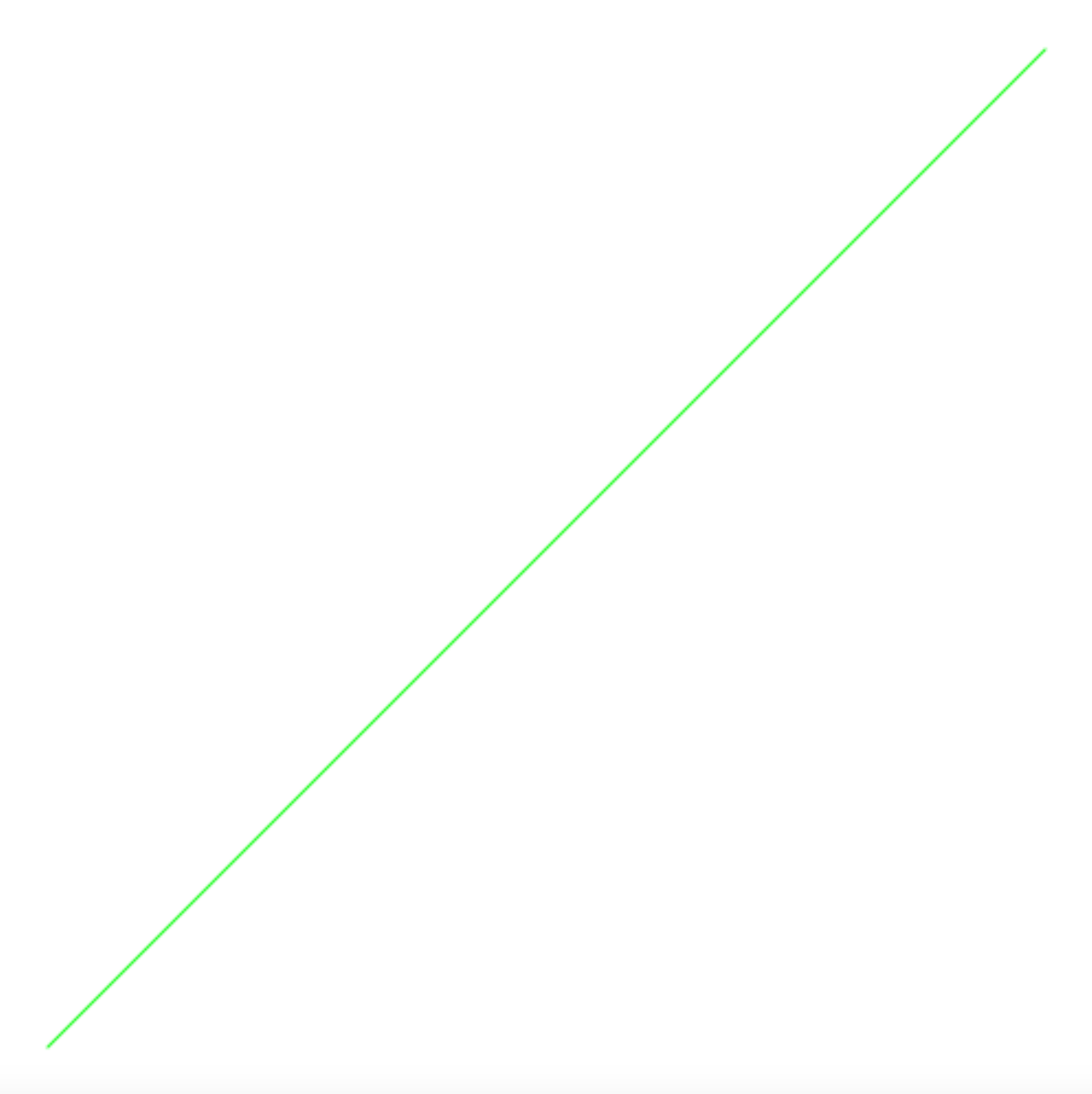
For example, the following function diagonal represents a
diagonal line
const diagonal = t => make_color_point(t, t, 0, 255, 0);
because it maps each value t to a point (t,t), which means
that x and y coordinates increase from the lower left to the
upper right.
The line is green because the “red” value is 0, the “green” value
is 255 (the maximum rgb value), and the “blue” value is 0.
The programs in this post are
available here;
to see the images, uncomment the lines that start with
//draw_connected_full_view....
You can visualize curves with the function draw_connected_full_view,
which takes a number n as argument and returns a function that
can be applied to a curve to visualize it. For that, the
curve is applied to n + 1 values, 0, 1, …, n, and the
resulting points displayed so that they all fit on the screen,
and are connected with each other with straight lines.
The following application draws the diagonal curve
by applying diagonal to the values 0, 0.25, 0.5, 0.75, and 1,
and the resulting points are connected.
draw_connected_full_view(4)(diagonal);
The Unit Circle
Similarly, you can draw a red circle using the trigonometric functions of sine and cosine:
const π = math_PI;
const unit_circle = t => make_color_point(
    math_cos(2 * π * t),                                       // x
    math_sin(2 * π * t),                                       // y
    255, 0, 0);                                              // rgb
draw_connected_full_view(100)(unit_circle);
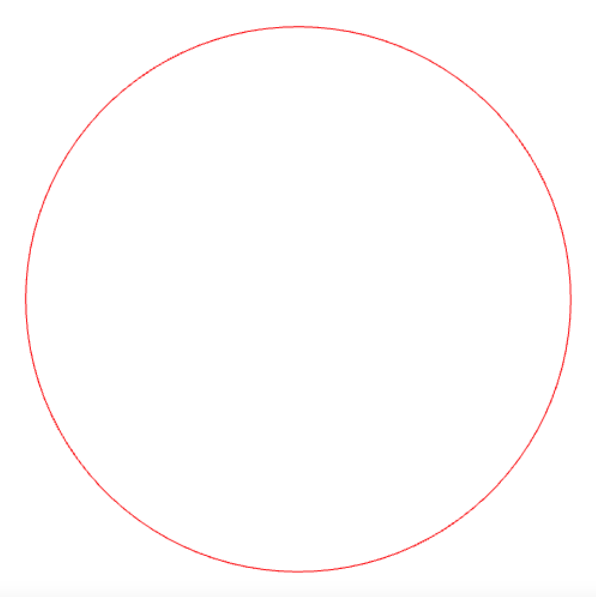
This circle is called the “unit circle” because it results from drawing a circle of radius 1 whose center has coordinate (0,0).
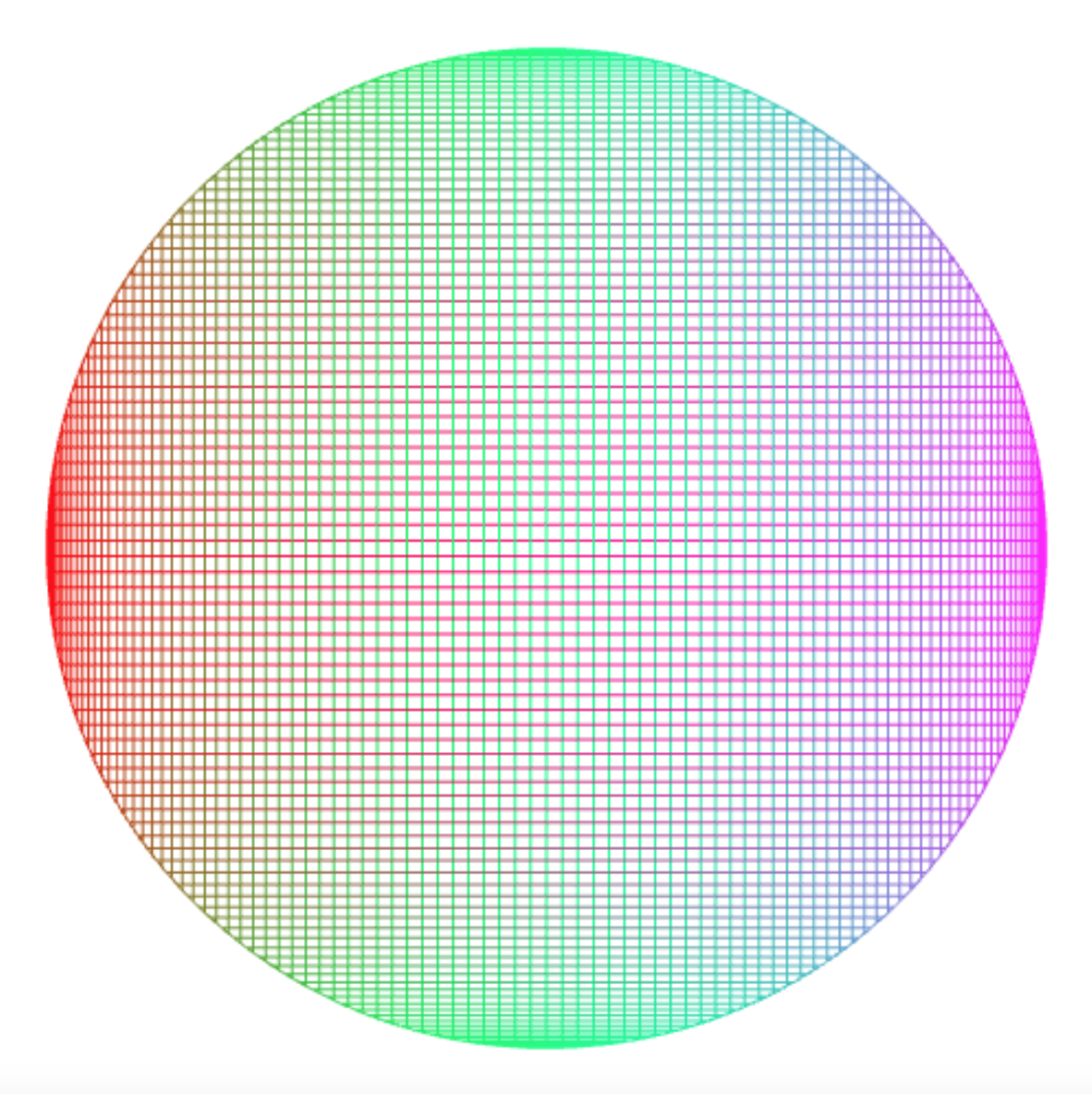
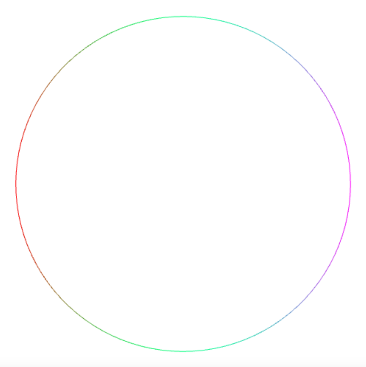
If you play with the rgb values, you can achieve a multi-colored unit circle:
const colored_unit_circle = t => make_color_point(
    math_cos(2 * π * t),                                       // x
    math_sin(2 * π * t),                                       // y
    math_pow(math_cos(2 * π * t), 2) * 255,                    // r
    math_pow(math_sin(2 * π * t), 2) * 255,                    // g
    math_pow(math_cos(    π * t), 2) * 255);                   // b
draw_connected_full_view(100)(colored_unit_circle);
In this post, I constrain myself to connecting points on this colored unit circle with straight lines, and turn this into an “art form”.
Connecting Points on the Unit Circle
The following abstraction connect_points comes in handy.
It takes a number n and a function f as arguments and connects
n points with each other. The points result from applying
the colored unit circle to values
f(0) / n, f(1) / n, …, f(n) / n
const connect_points =
    (n, f) =>
        draw_connected_full_view(n)
        (t => colored_unit_circle(f(math_round(t * n)) / n));
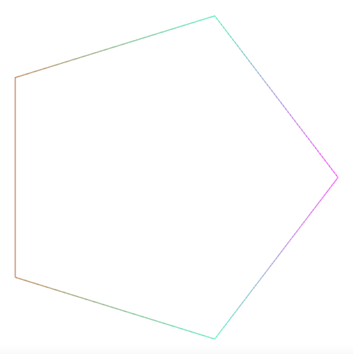
In the case where f is the identity function, you just
connect n points on the unit circle with each other, and
get a regular polygon with n vertices:
connect_points(5, k => k);
connecting the points
0 / n, 1 / n, 2 / n, …, n / n
The unit circle wraps around, if you apply it to values greater than 1, so you can obtain star shapes by connecting multiples of the given value.
connect_points(5, k => k * 2);
yields a pentagram
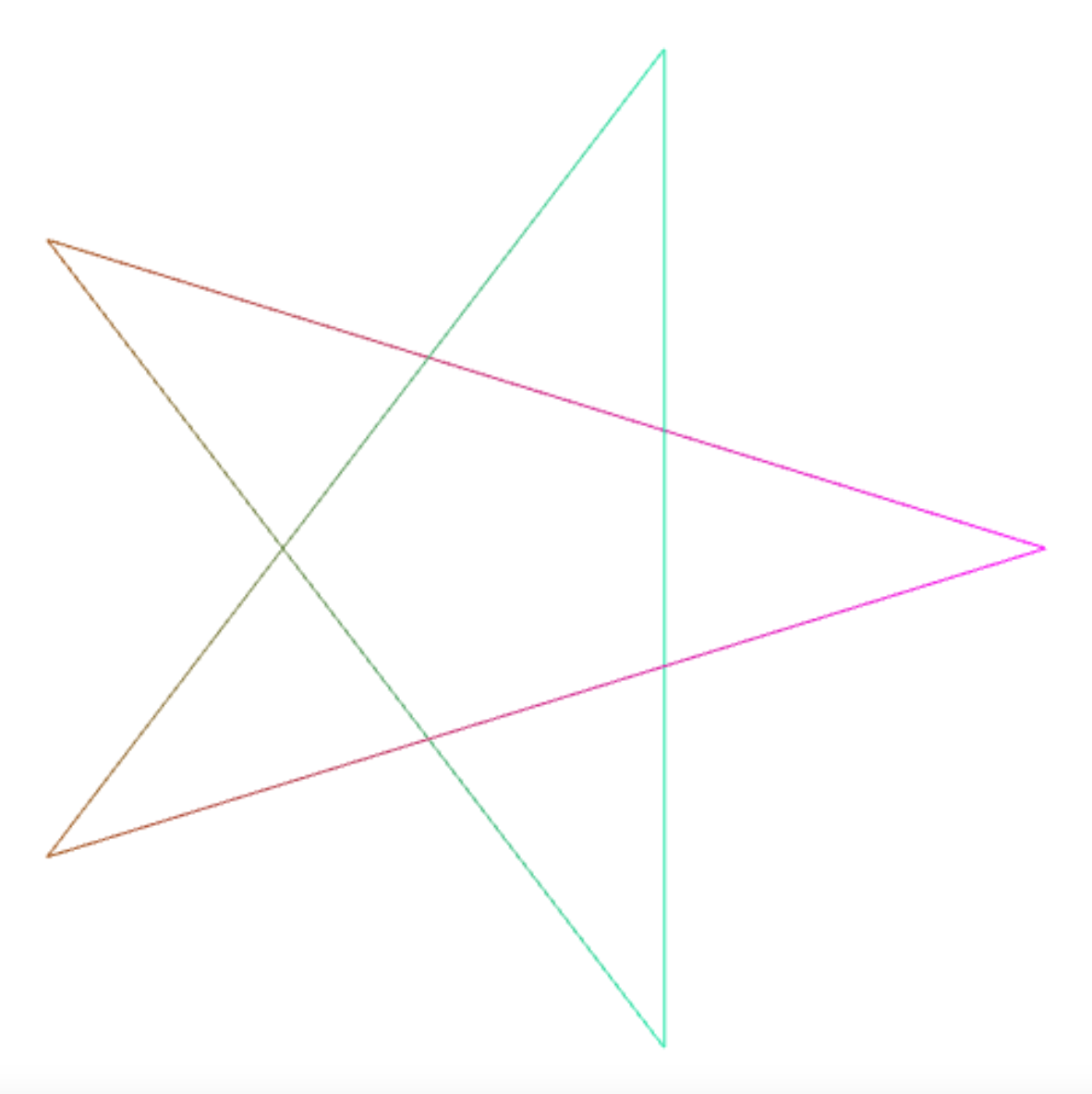
because you connect the points
0 / 5, 2 / 5, 4 / 5, 6 / 5, 8 / 5, and 10 / 5.
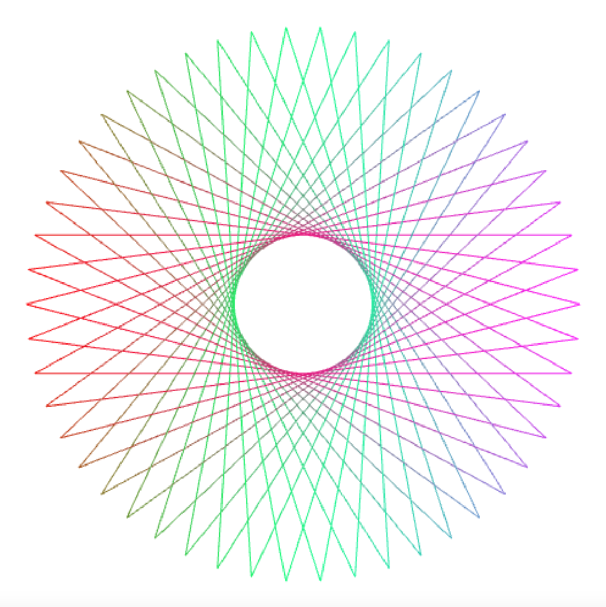
In the same way, you can create a star shape by connecting the corners of a 50-vertex polygon with each other such that each point is connected to the point 21 positions further, in counterclockwise direction:
connect_points(50, k => k * 21);
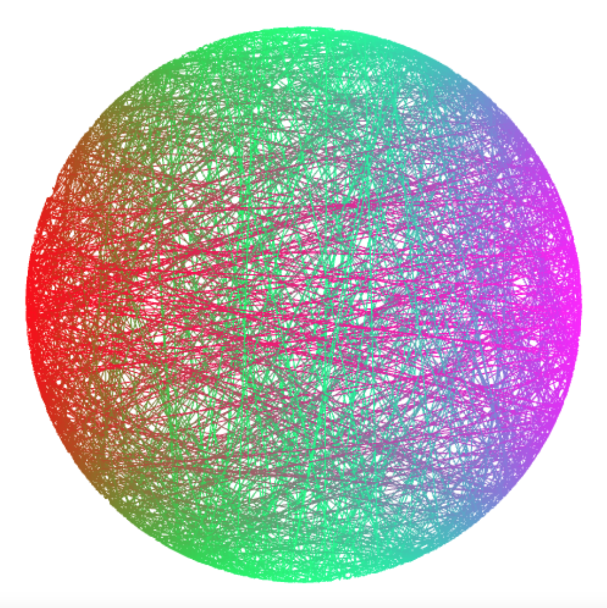
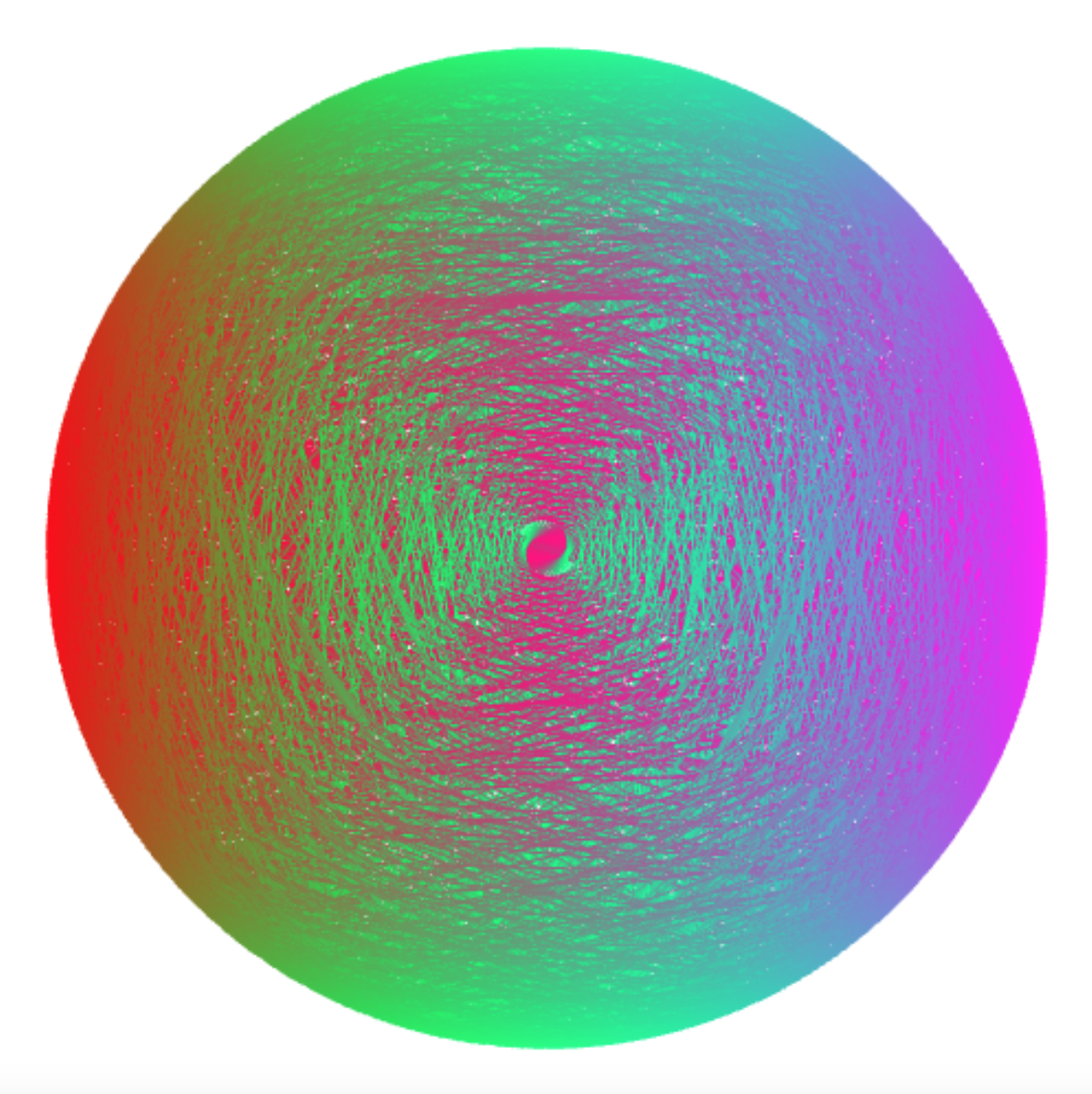
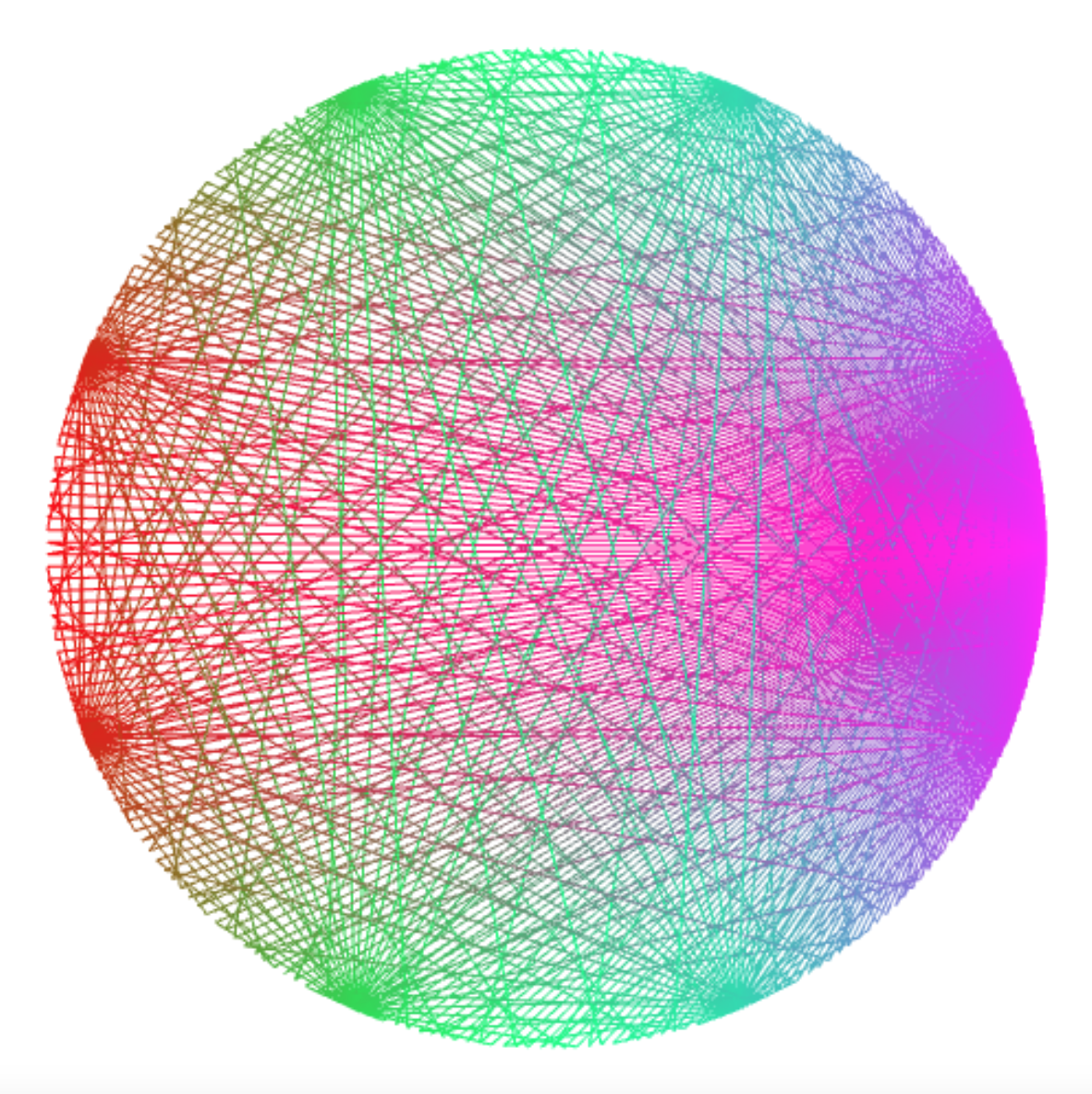
Choosing random values on the circle also leads to an intriguing pattern, when you choose n large enough:
connect_points(1000, k => 1000 * math_random());
Equation Signatures
Every equation seems to have a particular “signature” image in this art form. Here are some examples.
connect_points(6561, k => k * k );
connect_points(1024, k => k * k * k + 3 * k * k + 3 * k + 1);
connect_points(256, k => k * k * k * k);
connect_points(512, k => k * k * k * k);
connect_points(512, k => k * k * k * k * k);
connect_points(84, k => k * k * k * k * k * k * k);
Connecting Lines
Another way of connecting points on the unit circle using
a function f is to draw a line from i to f(i), for each i
from 0 to n. That can be accomplished using the connect_points
abstraction, by connecting (1) the point at i with (2) the
point at f(i), then (3) going back to i, which explains the
occurrences of the number 3 in the program.
const connect_lines =
    (n, g) =>
    connect_points(n * 3,
                   k => { const v = math_round((k - 1) / 3);
                          return k % 3 === 1 ? g(v) * 3 : v * 3; }
                  );
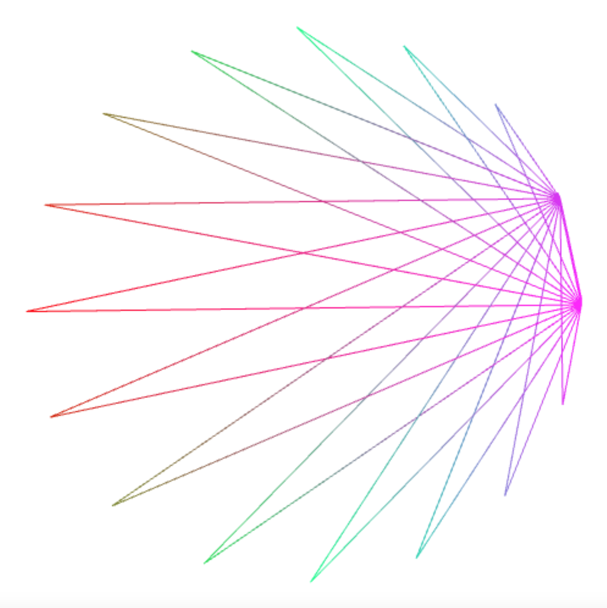
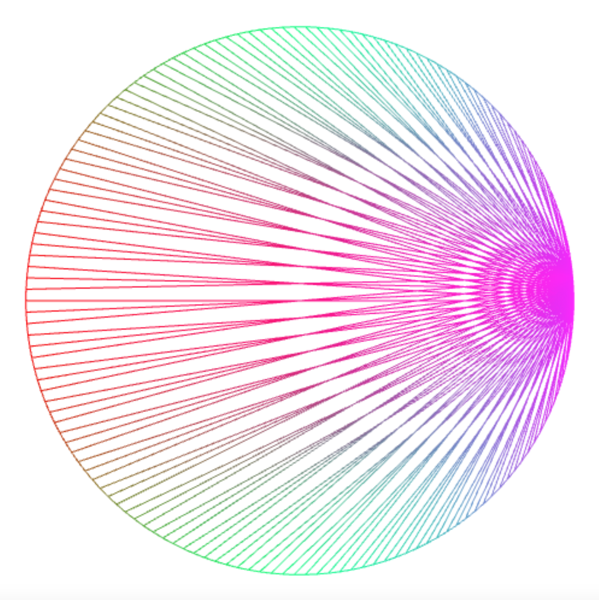
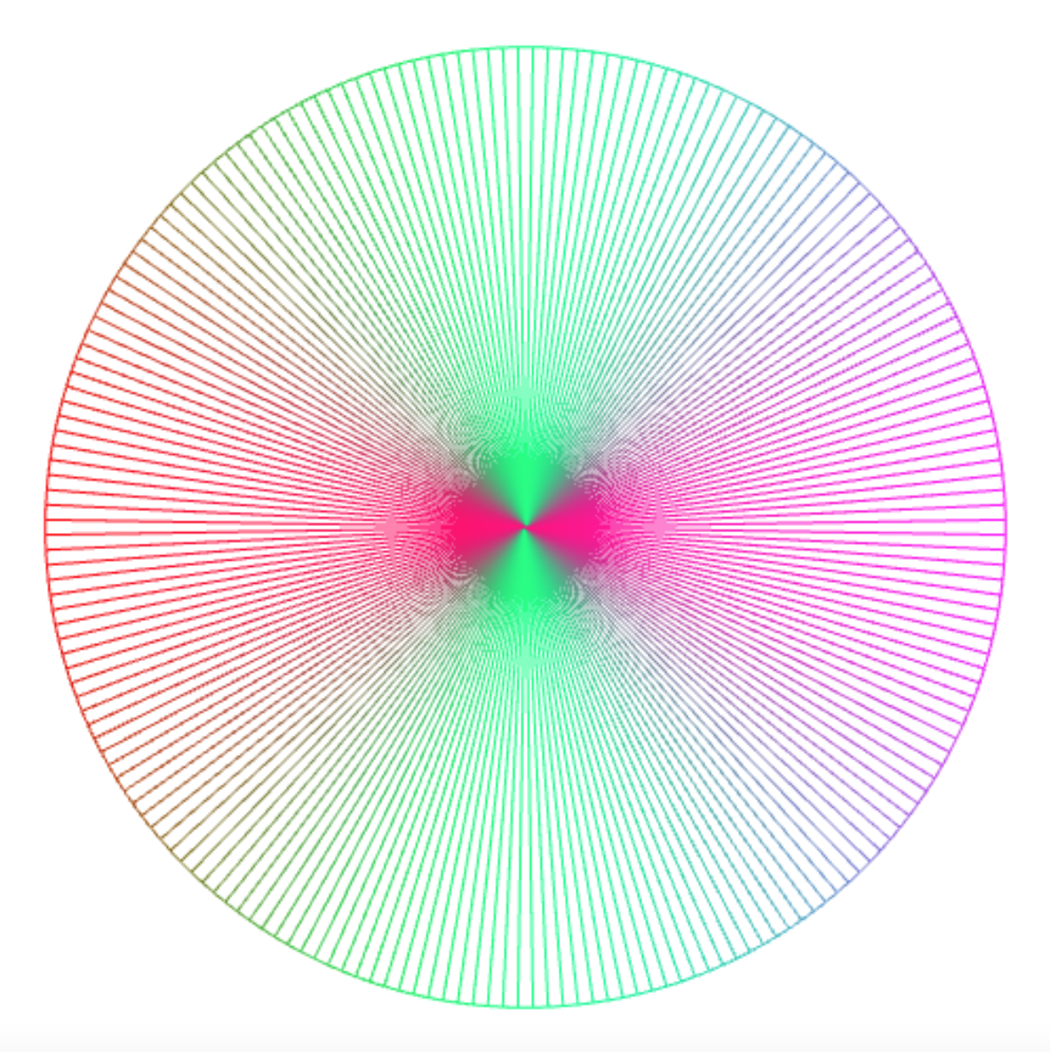
Connecting the every point with point 0 yields a picture like this.
connect_lines(150, k => 0);
which you can turn in counterclockwise direction by using a non-zero destination point, here point 25.
connect_lines(150, k => 25);
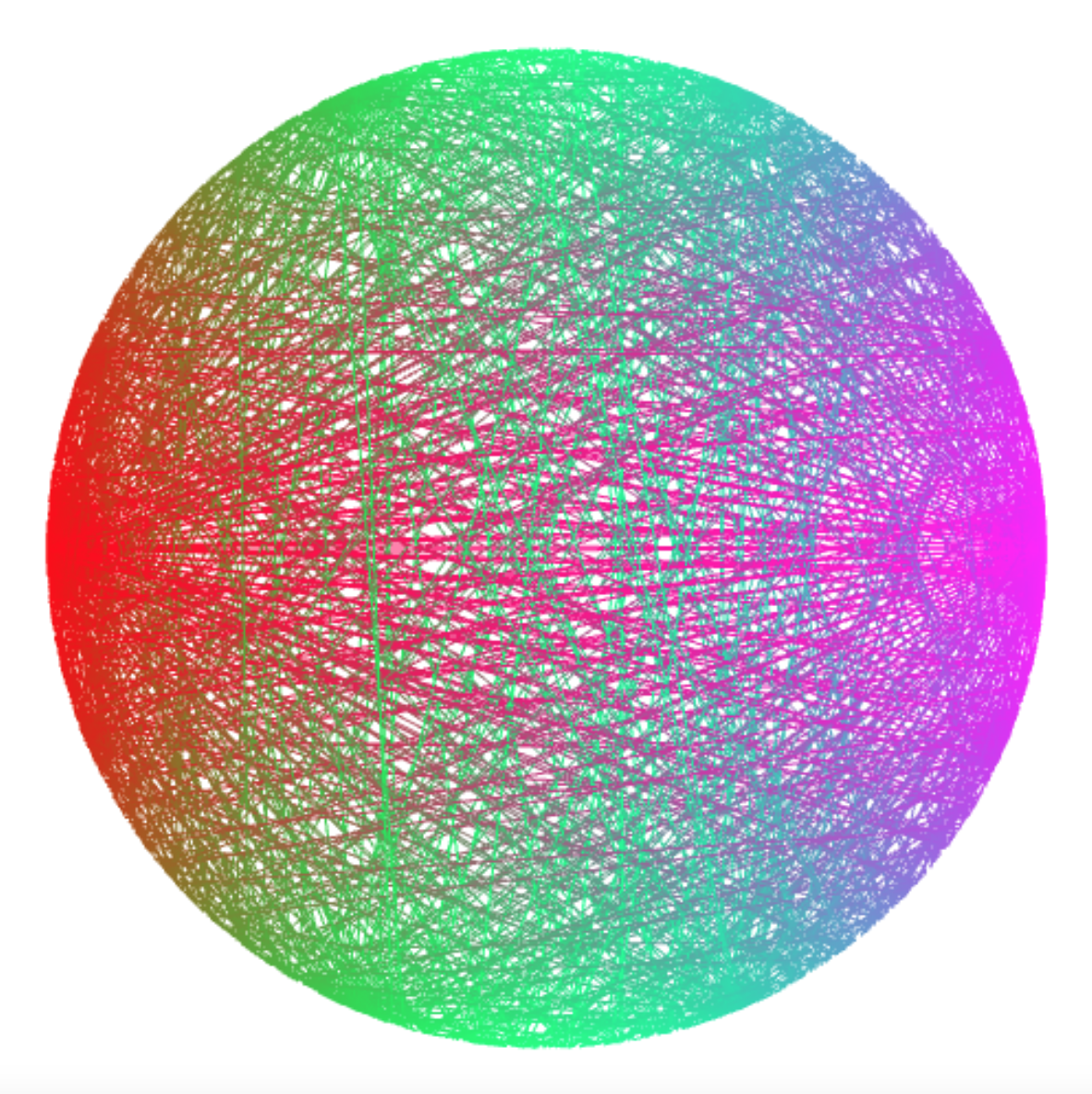
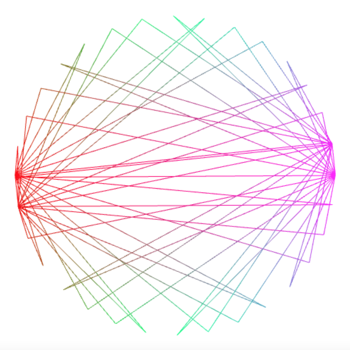
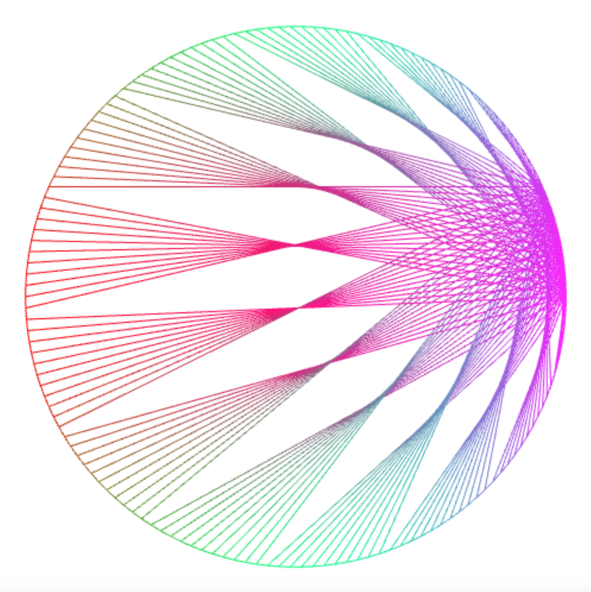
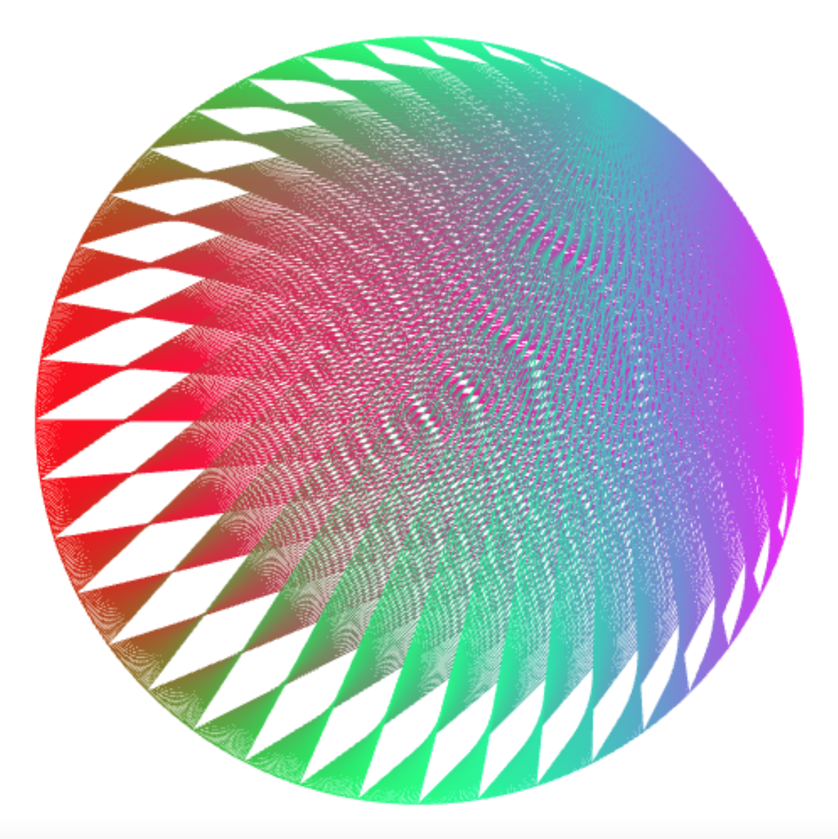
Connecting the points with a point that results from applying the modulo operator % yields intriguing interference patterns.
connect_lines(150, k => k % 3);
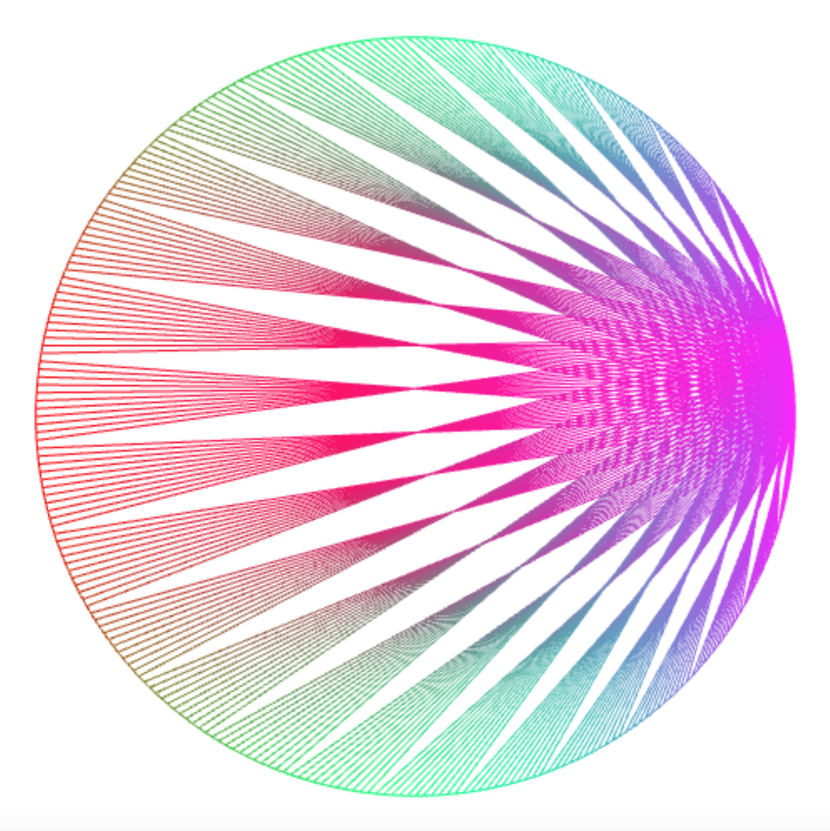
connect_lines(150, k => k % 11);
connect_lines(300, k => k % 11);
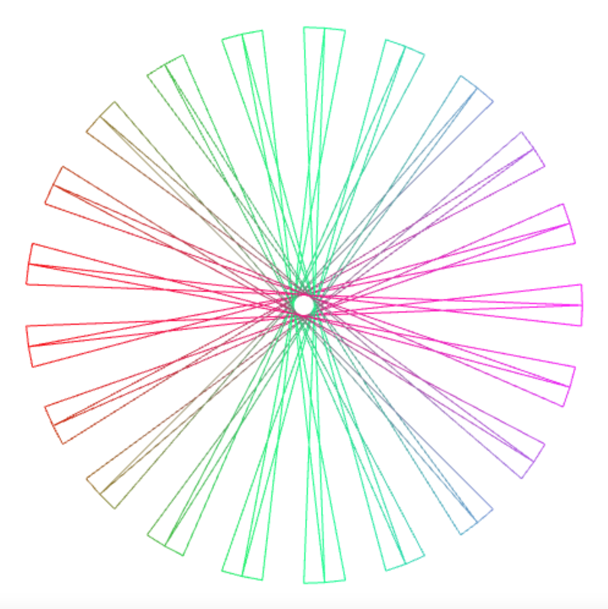
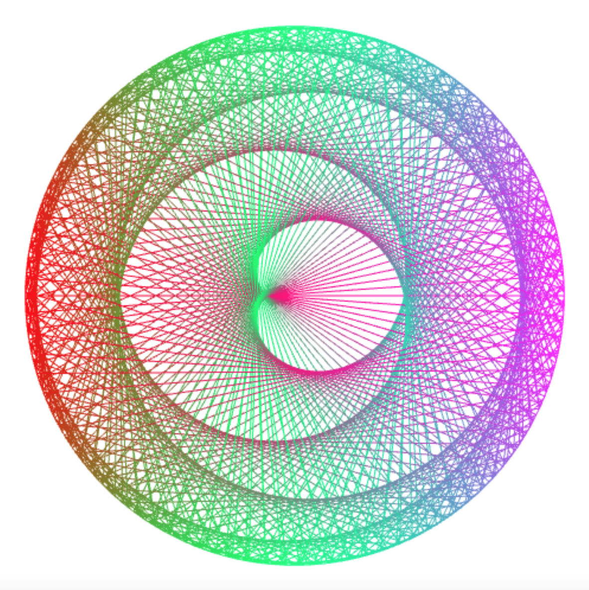
connect_lines(250, k => k % 11+160);
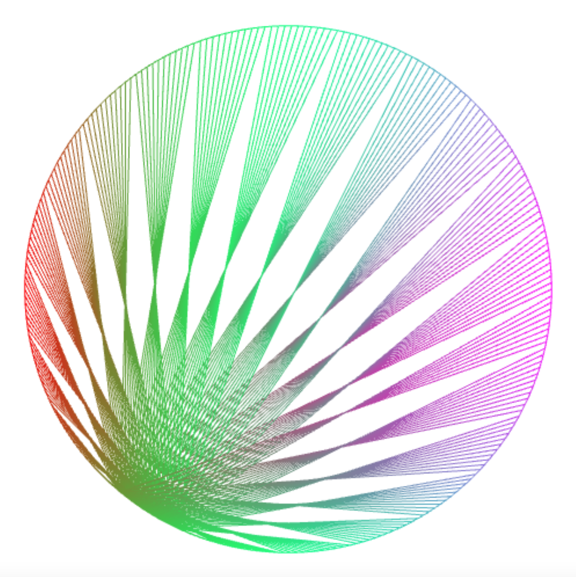
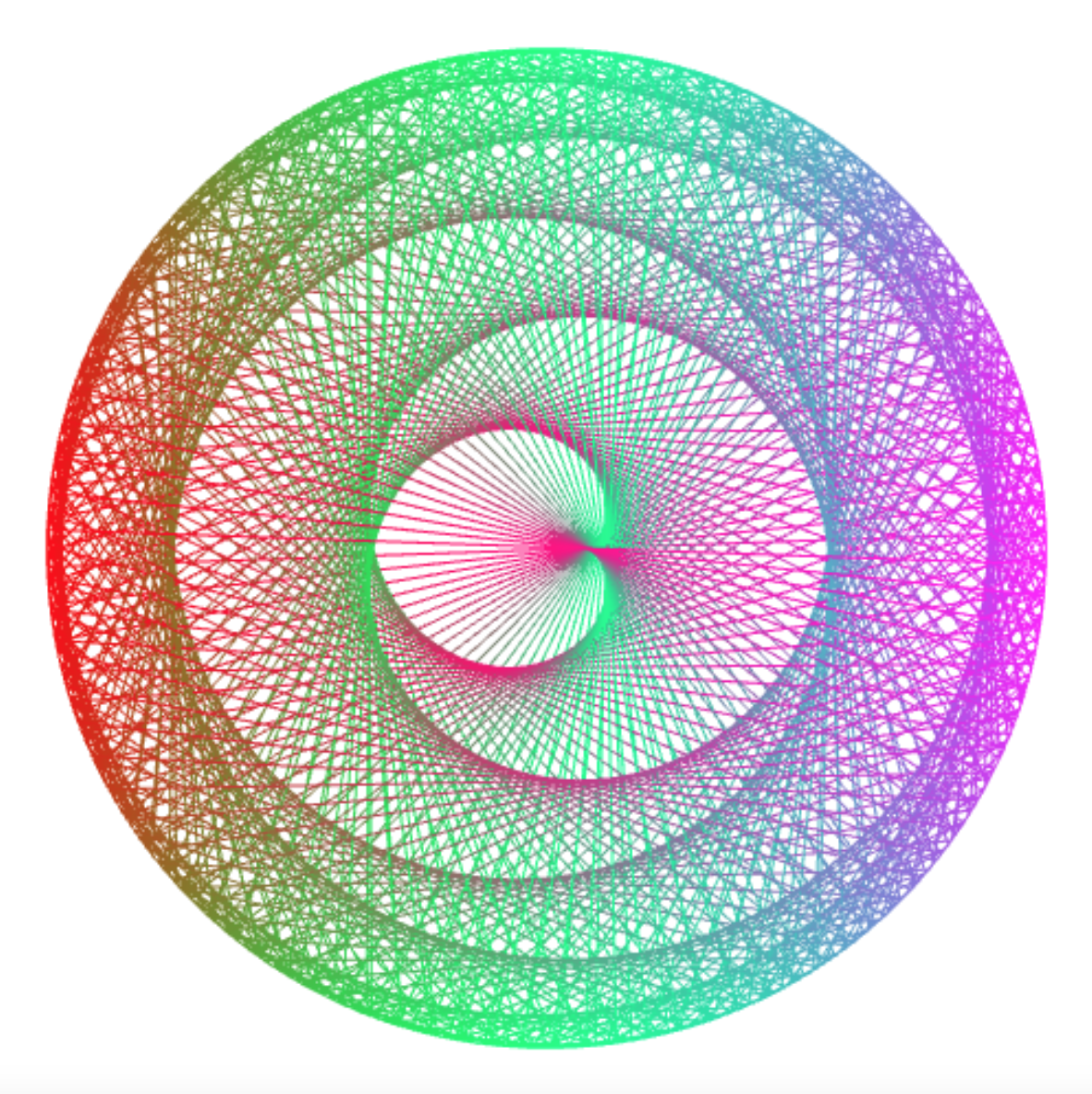
connect_lines(250, k => k % 10 + k / 10);
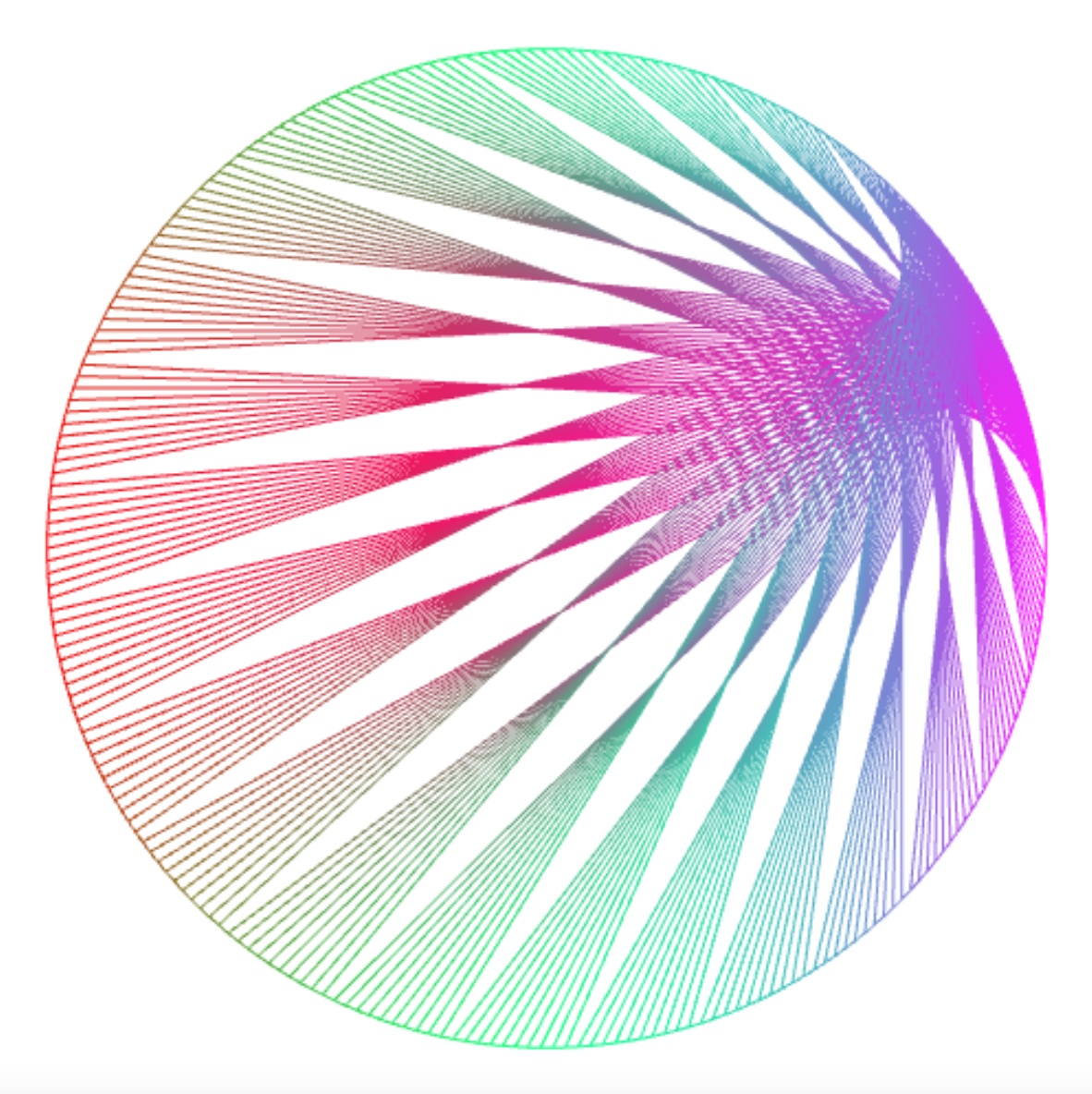
connect_lines(1000, k => k % 25 * 7);
Drawing Times Tables
Connecting points with their multiples leads to a visualization
of “times tables”. The Mathologer has
a video on this genre of unit circle art.
You can draw times tables with the abstraction draw_times_table:
const draw_times_table =
    (n, m) => connect_lines(n, k => k * m);
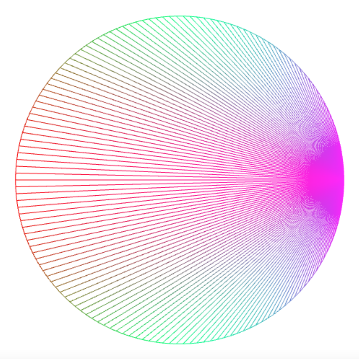
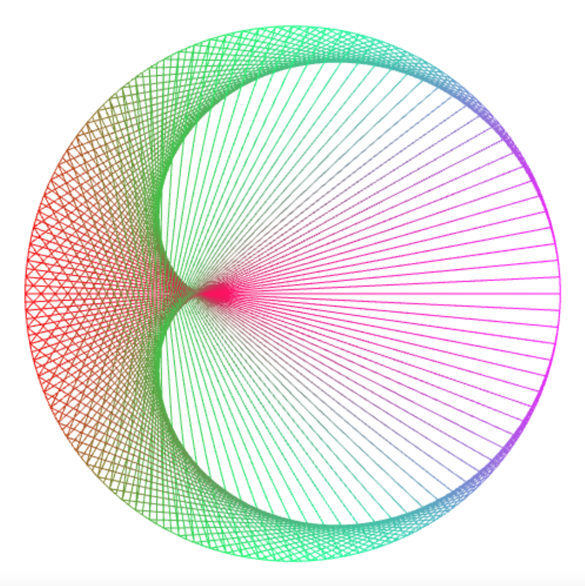
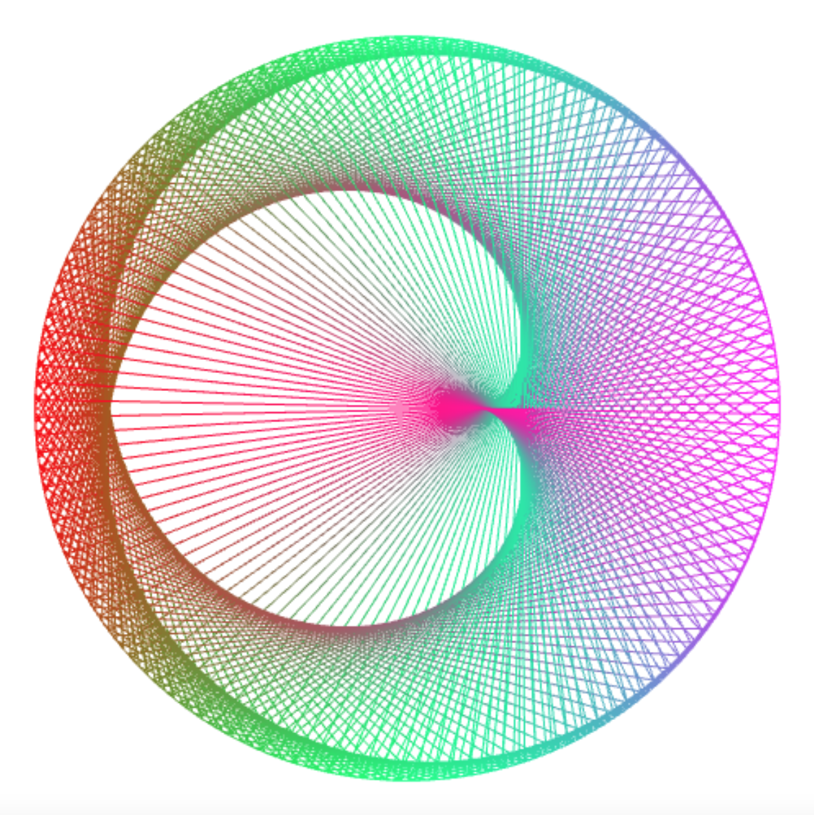
The times table for 2 is called the cardiod.
draw_times_table(200, 2); // m = 2: cardioid: 1 lobe
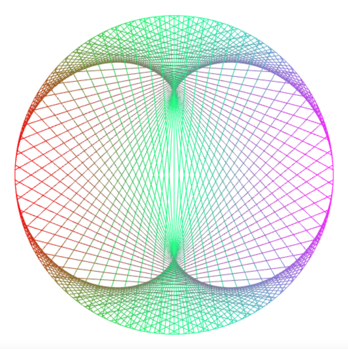
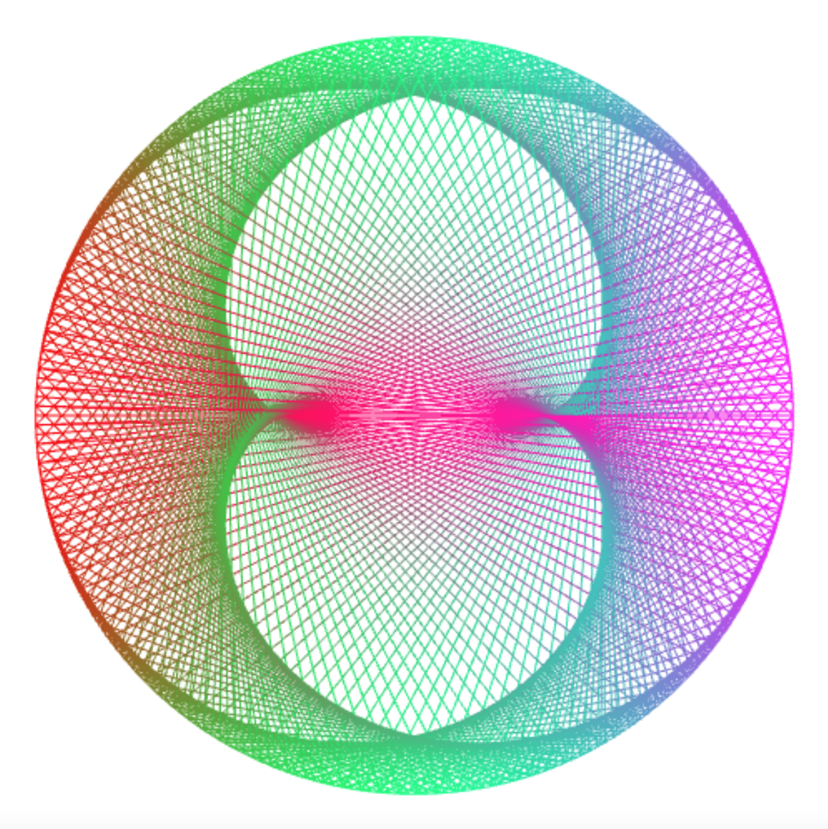
The times table for 3 is called the nephroid.
draw_times_table(200, 3); // m = 3: nephroid: 2 lobes
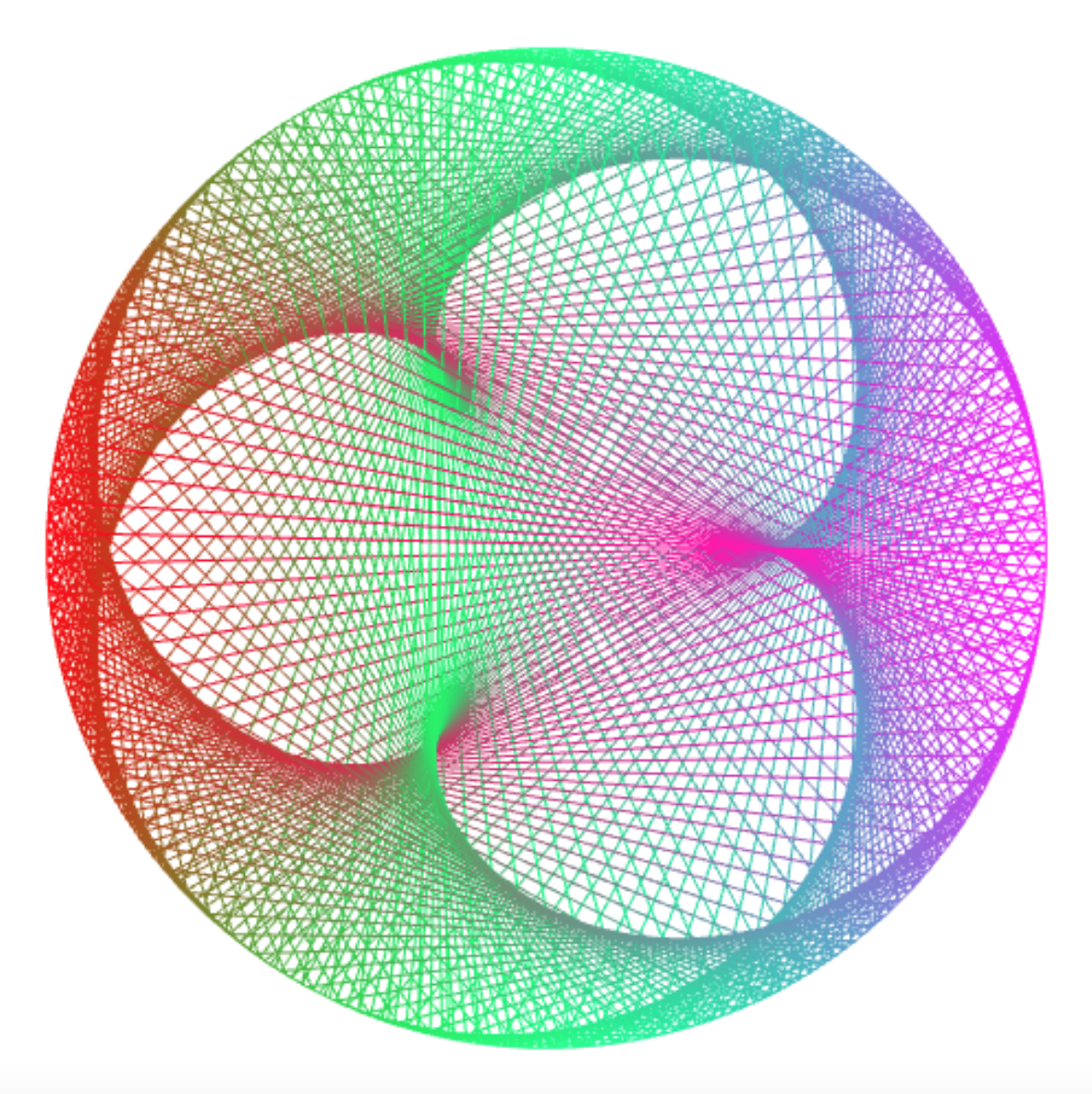
The number of “lobes” of the picture increases with m: For
m = 4 you get 3 lobes, etc.
draw_times_table(200, 4); // m = 4: 3 lobes...
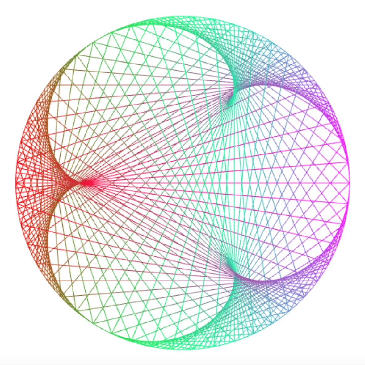
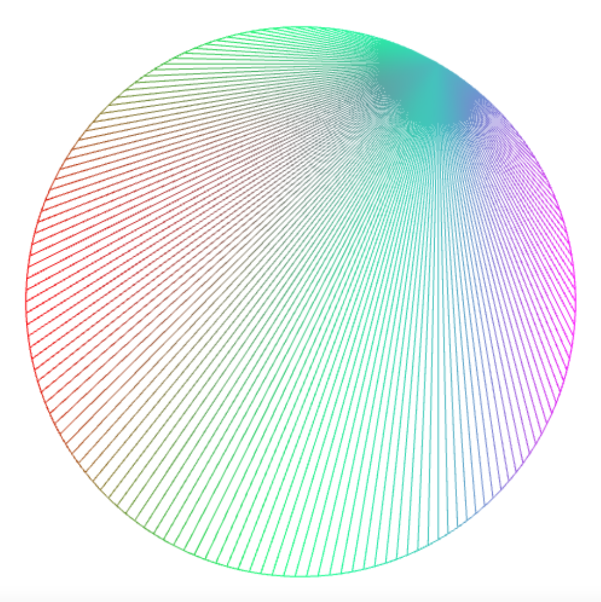
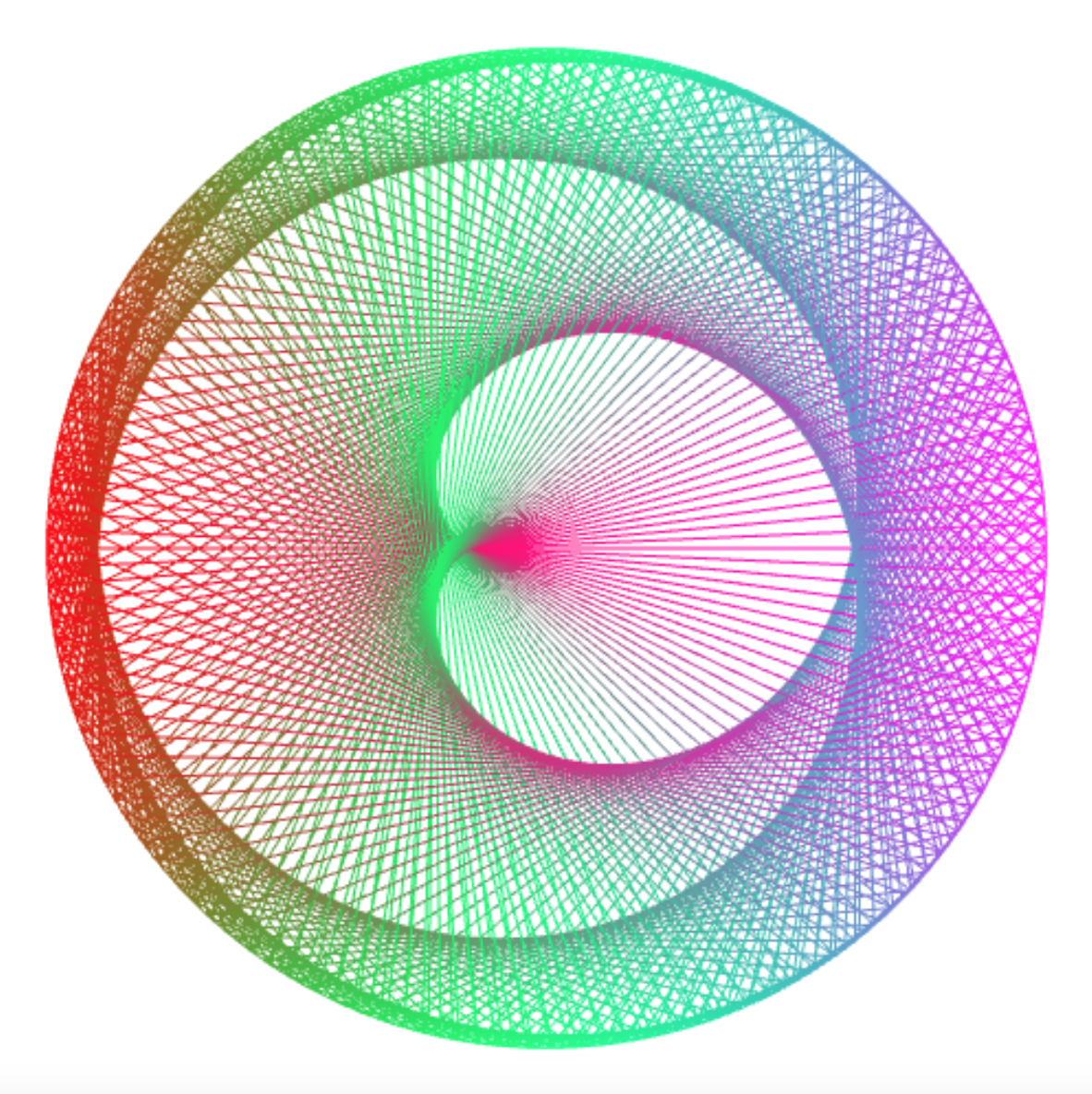
Specific relationships between n and m create interesting
visual patterns. For n = 397 and m = 200, you get a variant
of the cardiod…
draw_times_table(397, 200); // m = (n + 3) / 2: cardioid
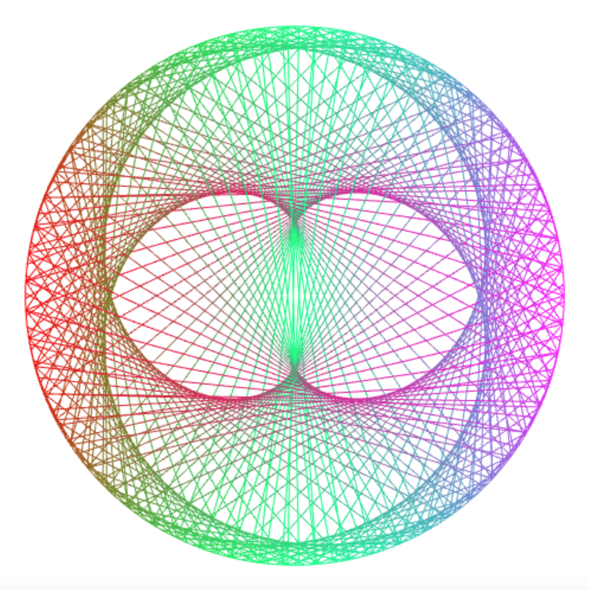
…and for n = 500 and m = 252, you get a variant of the
nephroid.
draw_times_table(500, 252); // m = (n + 4) / 2: nephroid
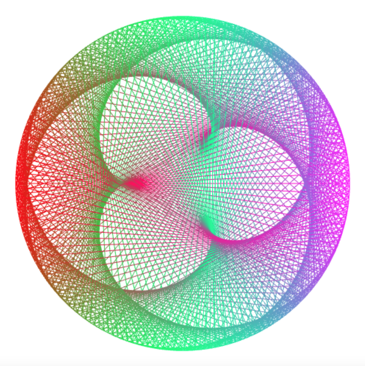
If you play with the numbers, you observe what relationship
between n and m gives rise to what kind of picture. Enjoy!
draw_times_table(501, 253); // m = (n + 5) / 2: 3 lobes...
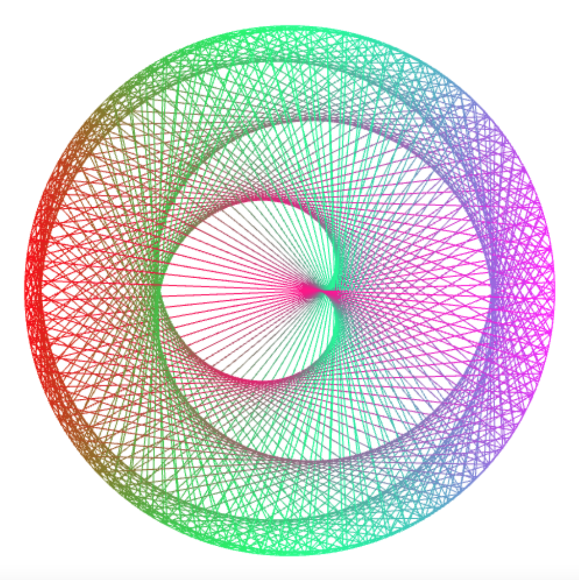
draw_times_table(500, 168); // m = (n + 4) / 3: cardioid
draw_times_table(295, 100); // m = (n + 5) / 3: nephroid
draw_times_table(594, 200); // m = (n + 6) / 3: 3 lobes...
draw_times_table(395, 100); // m = (n + 5) / 4: cardioid
draw_times_table(494, 100); // m = (n + 6) / 5: cardioid
draw_times_table(593, 100); // m = (n + 7) / 6: cardioid
draw_times_table(400, 201); // m = n / 2 + 1 (/4,/8,/16)
draw_times_table(400, 199); // m = (n / 2) - 1: square